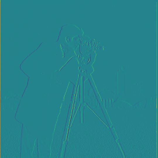
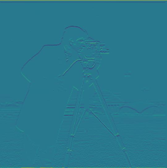
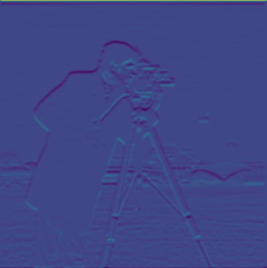
First, the cameraman image is convolved with Dx = [[1, -1]] and Dy = [[1], [-1]] respectively. Then, combine the Dx and Dy images by using
np.sqrt(dx_deriv ** 2 + dy_deriv ** 2), the result is called image gradient. Finally, binarized the image by setting the pixel value to 1 if it's above the threshold and 0 otherwise.
Results
Dx
Dy
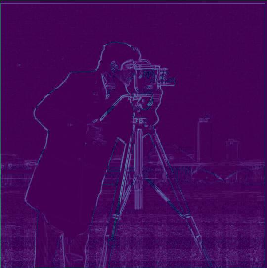
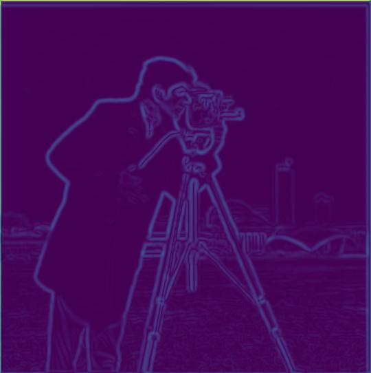
Image Gradient
combines Dx and Dy
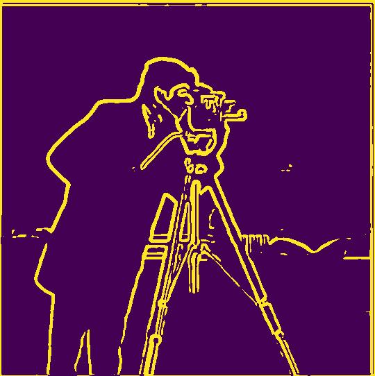
Image Gradient Binarized
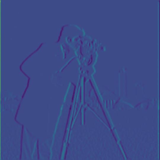
2.2 Derivative of Gaussian (DoG) Filter
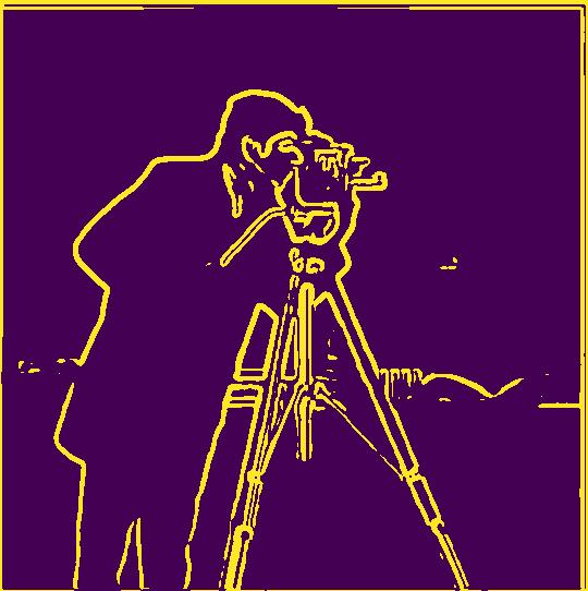
Method 1: First, apply the Gaussian filter to the image to get a blurred image. Then apply the same Dx, Dy, gradient computation and binarization
as in the previous section. The resulting edge image looks smoother and better better than the ones in section 1.1.
Method 2: Convolve Gaussian filter with Dx and Dy first, then apply the DoG (Derivative of Gaussian) to the original image.
After gradient computation and binarization, the result looks the same as the one in Method 1.
DoG Image Method 1
Convolve Guassian filter with Dx and Dy, then apply
the convolved filter onto the image
DoG Image Method 2
Apply the Gaussian filter to the image first, then convolve the filtered
image with Dx and Dy respectively.
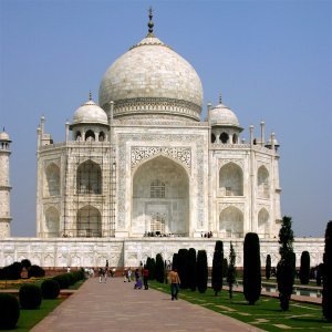
2.1 Image Sharpening
To sharpen an image, the image is convolved with a gaussian kernel, and the resulting image is denoted by img_blurred.
Then, the details of the image is computed as details = image - img_blurred. Lastly, detail is added back to the image, and the result is
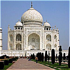
sharpened_image = image + alpha * details where alpha is a sharpening factor. Below is the before and after of the image "tal".
Before sharpening
After sharpening
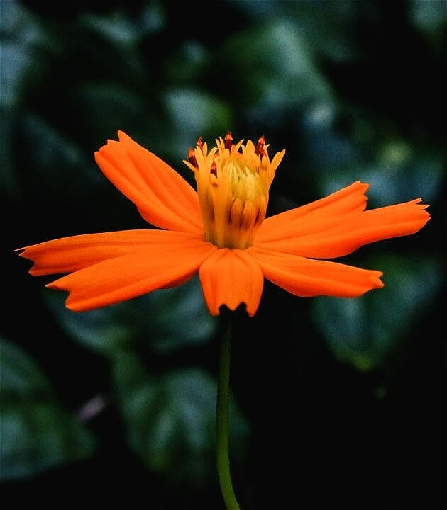
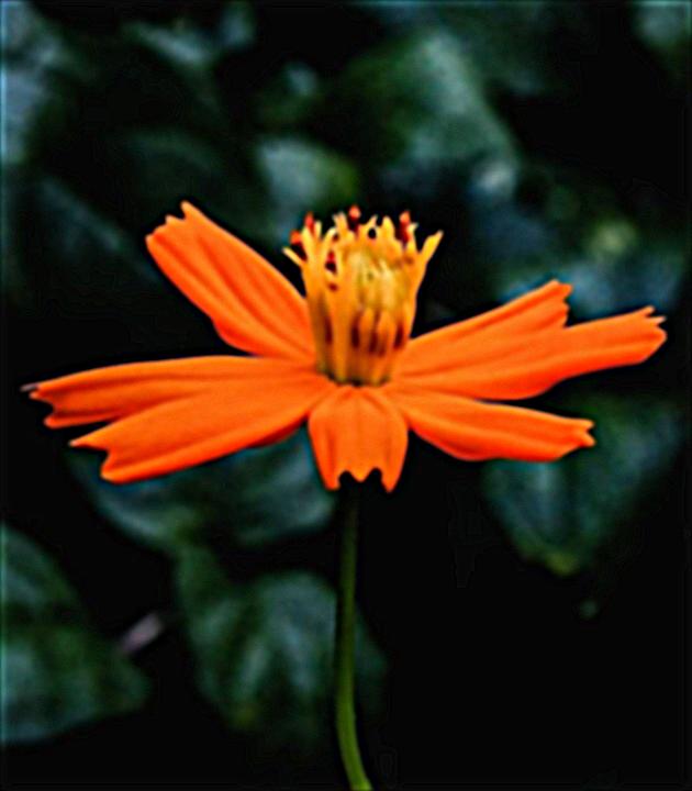
I also tested another image "flower". I blurred the image and then sharpened it. The result is as below
Original Image
Blurred Image
Sharpening the Blurred Image
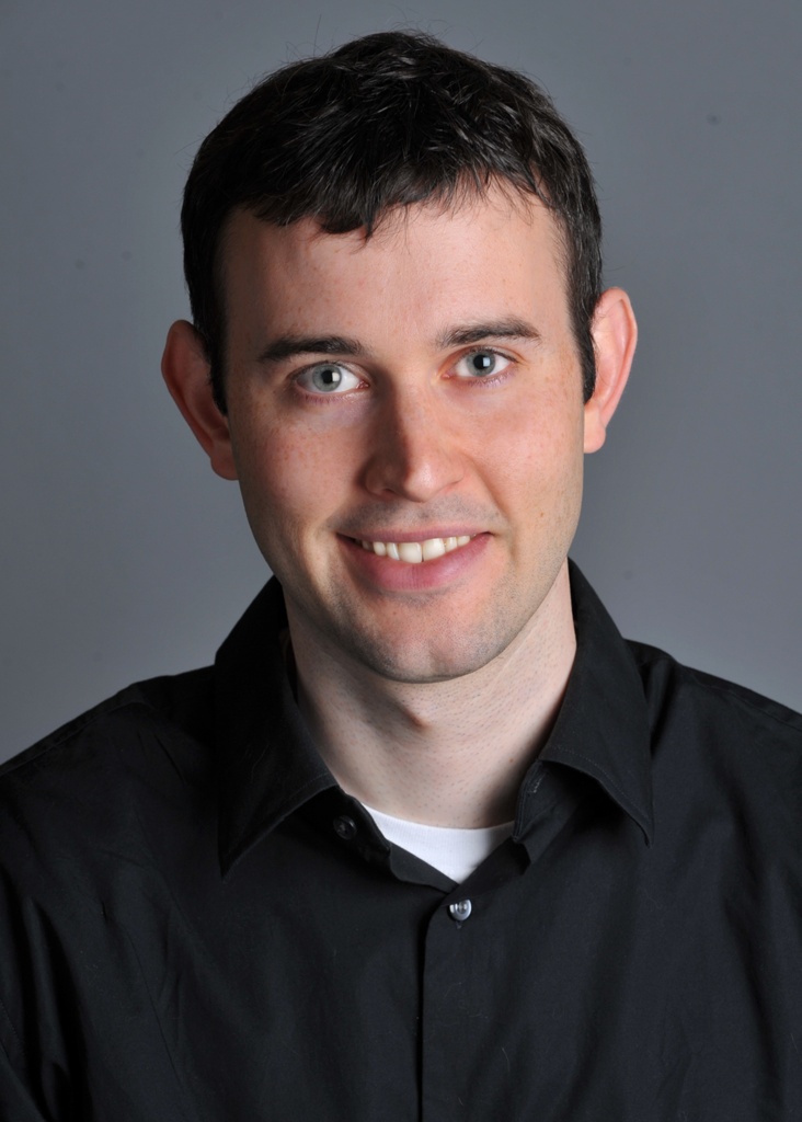
2.2 Hybrid Images
I implemented hybrid image algorithm according to the assignment: For the first image, filter out high frequency with
a Gaussian filter; for the second image, subtract the Gaussian-filtered image from the original. Then, add the filtered
first image and the filtered second image together to create the hybrid image. To test the algorithm, I used the
images provided by the assignment
Image 1
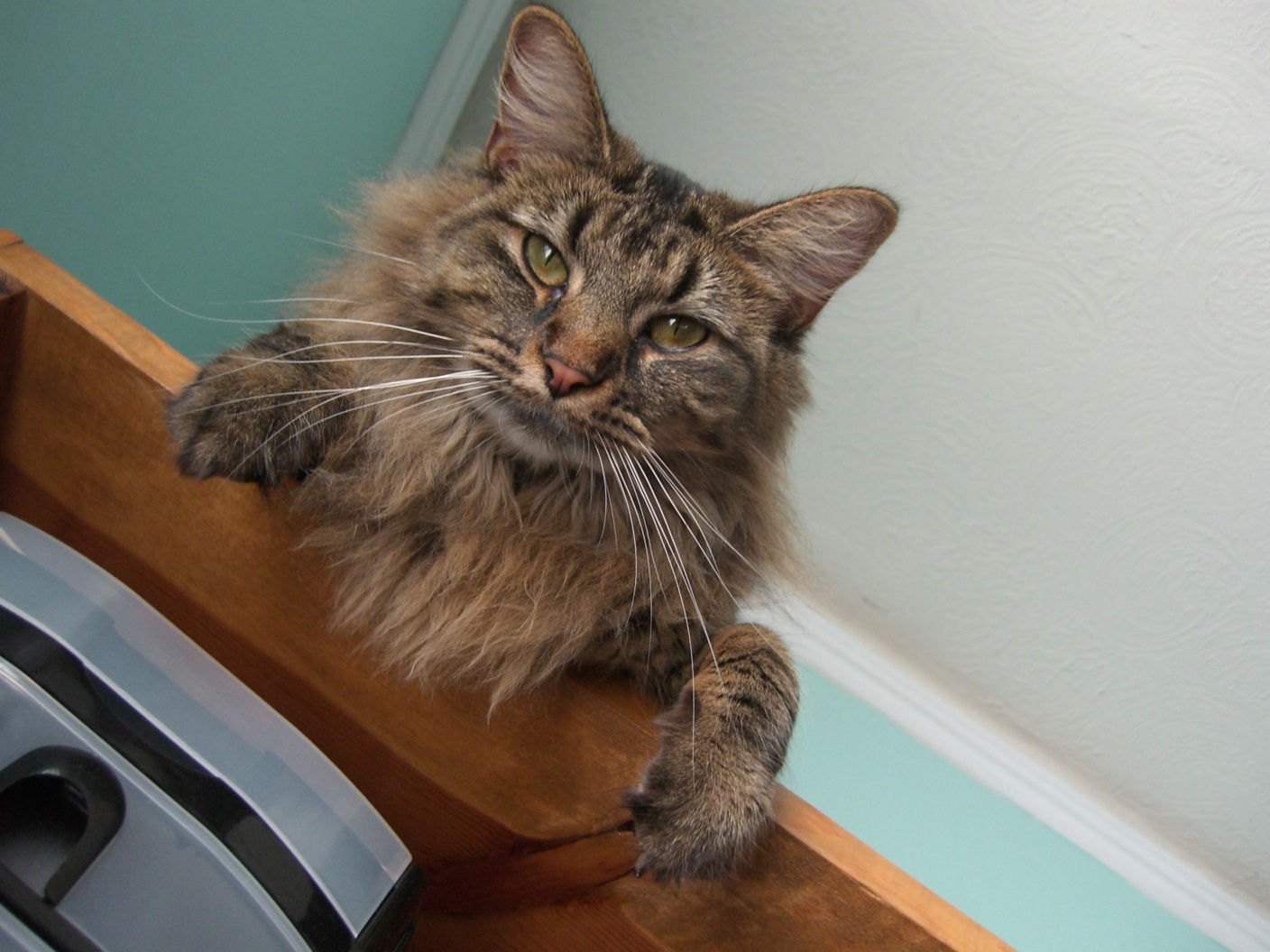
Image 2
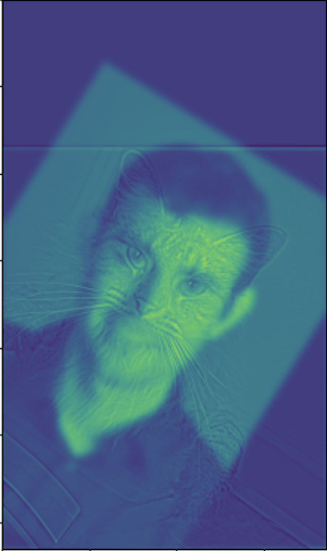
Hybrid Image
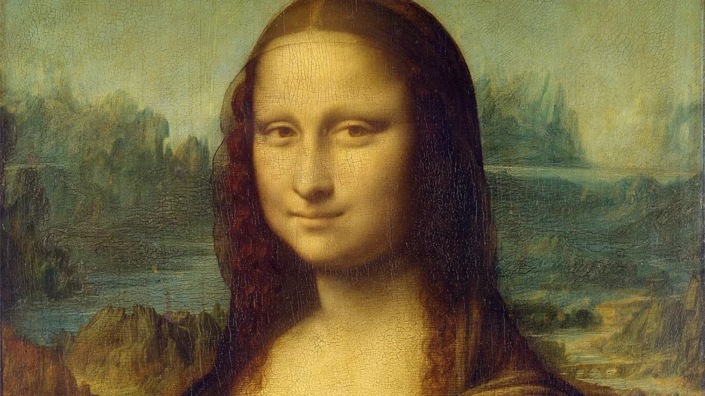
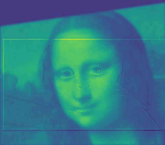
I also tested two other set of images. The first set is hybrid of Mona Lisa and a baby. This is considered success.
When you look close, Mona Lisa has big baby eyes. But when you look from far away, you see the original Mona Lisa.
Mona Lisa
Baby
Baby Mona Lisa
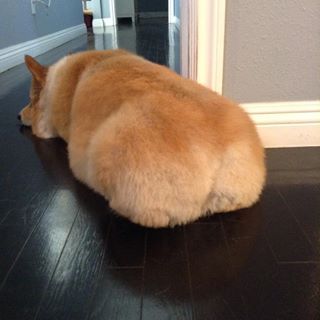
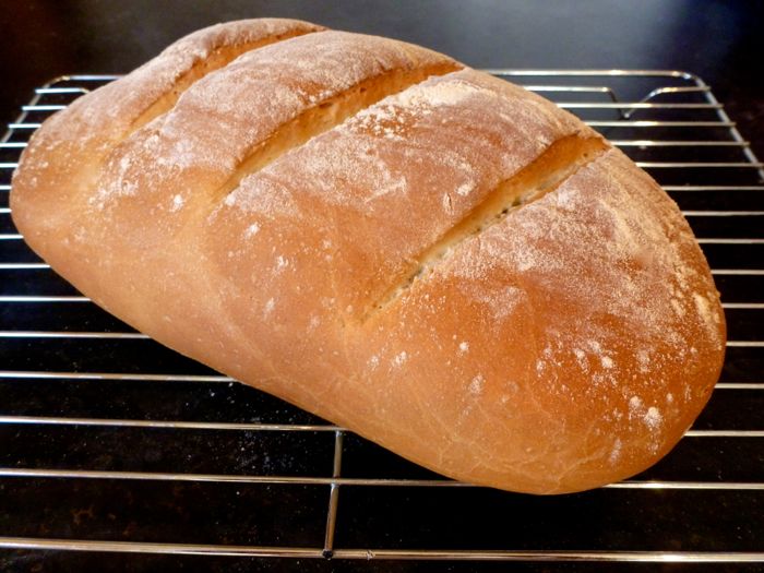
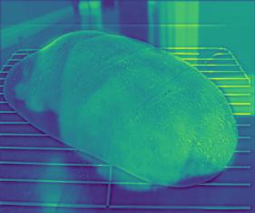
The other set of images is a bread and a corgi. This is kinda a failure: when you look close, you can see a bread, but Corgi
is also as obvious. I think this is because the graphic of a bread is too simple: it does not have many patterns
or features. On the other hand, the Corgi image is higher frequency and has many details, especially the texture of its fur.
A Corgi
A Bread
A Bread Corgi
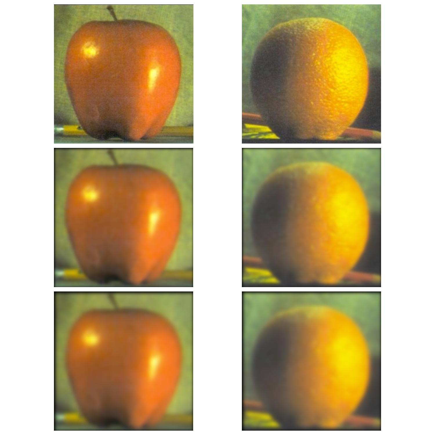
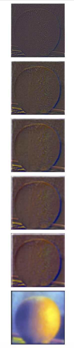
2.3 Gaussian and Laplacian Stacks
The Gaussian stack is created by repeatedly applying Gaussian filter to the image. Suppose the number of levels in
the Gaussian stack is N, then Laplacian stack is computed as
laplacian_stack[:,:, i] = gaussian_stack[:,:, i] - gaussian_stack[:, :, i+1] for 0 <= i <= N-2. At the last level N-1,
laplacian_stack[:,:, i] = gaussian_stack[:,:, i]
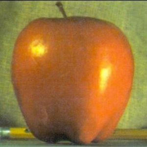
apple
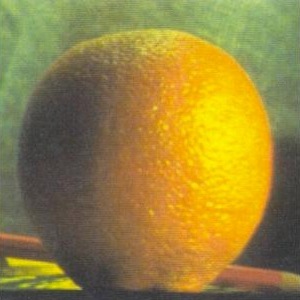
orange
Gaussian Stack
showing levels from 0 to 5
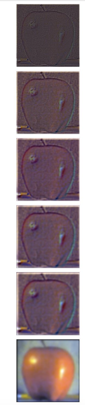
Laplacian Stack of Apple
showing levels from 0 to 5
Laplacian Stack of Orange
showing levels from 0 to 5
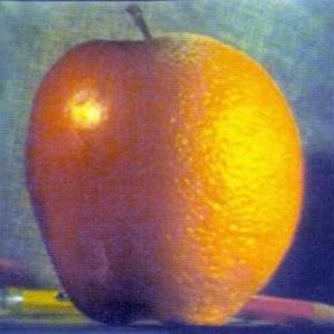
2.4 Multiresolution Blending
First, for the two input images img_1 and img_2, generate two laplacian stacks denoted as img_1_laplacian_stack and
img_2_laplacian_stack. Then select a mask g_mask, and create a gaussian stack of g_mask. The gaussian stack of the g_mask,
denoted as g_mask_gaussian_stack has the same number of levels as the Laplacian stacks. The blended image is computed as
blended_image[:,:, i] = img_1_laplacian_stack[:,:,i]* g_mask_gaussian_stack[:,:i] + img_2_laplacian_stack[:,:,i] * (1 - g_mask_gaussian_stack[:,:i])
For the apple and orange images, the blended image "oraple" is shown as the below